Immune Profiling of COVID-19 Severity: A Cross-Sectional Analysis#
Dataset: Stephenson et al., Nature Medicine 2021 (E-MTAB-10026)
Background#
Stephenson et al. profiled peripheral blood mononuclear cells (PBMCs) from COVID-19 patients across severity groups and timepoints, providing insights into immune dynamics during disease progression.
Important Methodological Notes#
This is an OBSERVATIONAL study, not a randomized trial:
Disease severity (Mild vs Severe) is an outcome, not a treatment assignment
Patients are not randomly assigned to severity groups
Differences between groups reflect disease biology, not causal treatment effects
We use sctrial’s infrastructure for structured comparisons, but interpret results as descriptive associations
Time axis considerations:
Days From Onset (DFO): Biological time since symptom onset - captures disease progression
Collection_Day: Calendar time since study enrollment - captures sampling schedule
These are fundamentally different; we use DFO for biological interpretability
Analysis strategy: Given limited longitudinal pairing in this dataset, we focus on cross-sectional comparisons between severity groups at each timepoint, which is the most statistically appropriate approach.
1. Setup and Configuration#
[1]:
# Imports - consolidated in one cell
import warnings
warnings.filterwarnings('ignore', category=FutureWarning)
# Note: We do NOT suppress UserWarning — sctrial issues important
# statistical caveats (e.g. low-cluster reliability) as UserWarnings.

import numpy as np
import pandas as pd
import scipy.sparse as sp
import matplotlib.pyplot as plt
import seaborn as sns
import scanpy as sc
import statsmodels.formula.api as smf
from statsmodels.stats.multitest import multipletests
from scipy.stats import mannwhitneyu  # Import here for use across notebook
from pathlib import Path
import urllib.request

import sctrial as st
import itertools

# Configuration constants
MIN_GENES_FOR_SCORE = 5
MIN_PARTICIPANTS_FOR_COMPARISON = 5
MIN_CELLS_PER_CELLTYPE = 100
SEED = 42
FDR_ALPHA = 0.25  # Exploratory threshold; use 0.05 for confirmatory analyses

pd.options.mode.chained_assignment = None
print(f"sctrial version: {st.__version__ if hasattr(st, '__version__') else 'dev'}")


def _fmt_fdr(v):
    """Format FDR/p-value: scientific notation for very small values."""
    return f"{v:.2e}" if v < 0.001 else f"{v:.3f}"
sctrial version: 0.3.3
2. Data Loading and Processing#
[2]:
# Dataset loaders and helpers
# All available at top-level: st.load_stephenson_data, st.count_paired, st.categorize_celltype
from sctrial.datasets import load_stephenson_data, count_paired, categorize_celltype
[3]:
# Load data
adata = load_stephenson_data(force_reprocess=False)

print("\n=== Dataset Summary ===")
print(f"Cells: {adata.n_obs:,}")
print(f"Genes: {adata.n_vars:,}")
print(f"Severity groups: {adata.obs['severity'].unique().tolist()}")
print(f"DFO bins: {sorted(adata.obs['dfo_bin'].unique().tolist())}")
print(f"Cell types: {adata.obs['celltype'].nunique()}")
print(f"Participants: {adata.obs['participant_id'].nunique()}")
=== Dataset Summary ===
Cells: 205,202
Genes: 24,929
Severity groups: ['Severe', 'Mild']
DFO bins: ['DFO_0-7', 'DFO_15+', 'DFO_8-14']
Cell types: 50
Participants: 34
/var/folders/71/dc4p4yz15s74z9c69xy6sk_00000gt/T/ipykernel_52813/900064142.py:2: UserWarning: Cached file lacks processing_params metadata; cannot verify it matches current settings. Consider reprocessing with force_reprocess=True.
  adata = load_stephenson_data(force_reprocess=False)
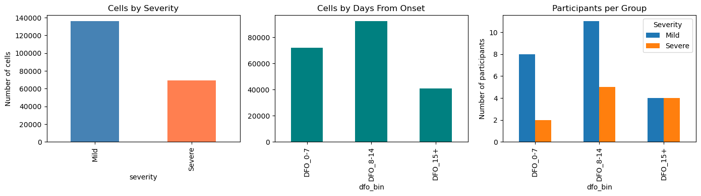
3. Sample Size Assessment#
Before analysis, we assess sample sizes to determine appropriate statistical methods.
[4]:
# Sample sizes by severity and timepoint
sample_sizes = (
    adata.obs
    .groupby(["severity", "dfo_bin"], observed=True)["participant_id"]
    .nunique()
    .unstack(fill_value=0)
)
print("Participants per severity × DFO bin:")
display(sample_sizes)

# Check for longitudinal pairing

dfo_visits = ["DFO_0-7", "DFO_8-14"]
n_paired_dfo = count_paired(adata.obs, "dfo_bin", dfo_visits)

print("")
print(f"Longitudinal pairing (DFO 0-7 → 8-14): {n_paired_dfo} participants")

if n_paired_dfo < MIN_PARTICIPANTS_FOR_COMPARISON:
    print("")
    print(f"⚠️  WARNING: Only {n_paired_dfo} paired participants available.")
    print("   Difference-in-Differences analysis requires ≥5 paired participants.")
    print("   This notebook will focus on CROSS-SECTIONAL comparisons instead.")
    CAN_DO_DID = False
else:
    CAN_DO_DID = True

# Visualize sample sizes
fig, axes = plt.subplots(1, 3, figsize=(14, 4))

# Cells by severity
adata.obs["severity"].value_counts().plot(
    kind="bar", ax=axes[0], color=["steelblue", "coral"]
)
axes[0].set_title("Cells by Severity")
axes[0].set_ylabel("Number of cells")

# Cells by DFO
adata.obs["dfo_bin"].value_counts().sort_index().plot(
    kind="bar", ax=axes[1], color="teal"
)
axes[1].set_title("Cells by Days From Onset")

# Participants per group
sample_sizes.T.plot(kind="bar", ax=axes[2])
axes[2].set_title("Participants per Group")
axes[2].set_ylabel("Number of participants")
axes[2].legend(title="Severity")

plt.tight_layout()
plt.show()
Participants per severity × DFO bin:
| dfo_bin | DFO_0-7 | DFO_8-14 | DFO_15+ |
|---|---|---|---|
| severity | |||
| Mild | 8 | 11 | 4 |
| Severe | 2 | 5 | 4 |
Longitudinal pairing (DFO 0-7 → 8-14): 0 participants

⚠️  WARNING: Only 0 paired participants available.
   Difference-in-Differences analysis requires ≥5 paired participants.
   This notebook will focus on CROSS-SECTIONAL comparisons instead.
4. Study Design Configuration#
We configure the comparison structure. Note: We use sctrial’s TrialDesign for convenience, but this is an observational comparison, not a randomized trial.
[5]:
# Add log1p-CPM normalization
if "log1p_cpm" not in adata.layers:
    adata = st.add_log1p_cpm_layer(adata, counts_layer="counts", out_layer="log1p_cpm")
    print("Added log1p_cpm layer")

# Define comparison design
# Note: We call Severe the "treated" group for sctrial compatibility,
# but this is purely for software purposes - there is no treatment!
design = st.TrialDesign(
    participant_col="participant_id",
    visit_col="dfo_bin",
    arm_col="severity",
    arm_treated="Severe",   # Reference group for comparison
    arm_control="Mild",
    celltype_col="celltype",
)

# Available visits for analysis
available_visits = sorted(adata.obs["dfo_bin"].unique().tolist())
print(f"Available DFO bins: {available_visits}")

# Covariates - match actual column names in the dataset
covariate_mapping = {
    "Age_interval": "age",
    "Sex": "sex",
    "Site": "site",
    "Smoker": "smoker",
}
covariates = [c for c in covariate_mapping.keys() if c in adata.obs.columns]
print(f"Available covariates: {covariates}")

# Check covariate distributions
if covariates:
    print("\nCovariate summary by severity:")
    for cov in covariates[:3]:  # Show first 3
        print(f"\n{cov}:")
        print(adata.obs.groupby("severity")[cov].value_counts().unstack(fill_value=0))

design
Added log1p_cpm layer
Available DFO bins: ['DFO_0-7', 'DFO_15+', 'DFO_8-14']
Available covariates: ['Age_interval', 'Sex', 'Site', 'Smoker']

Covariate summary by severity:

Age_interval:
Age_interval  (20, 29]  (30, 39]  (40, 49]  (50, 59]  (60, 69]  (70, 79]  \
severity
Mild              7446     16252     22525     21651     35854     17798
Severe               0      5589     15433     32828      4164      2233

Age_interval  (80, 89]  (90, 99]
severity
Mild             14410         0
Severe            9019         0

Sex:
Sex       Female   Male
severity
Mild       84262  51674
Severe     49556  19710

Site:
Site      Cambridge    Ncl  Sanger
severity
Mild          26277  87676   21983
Severe         6397  44275   18594
[5]:
TrialDesign(participant_col='participant_id', visit_col='dfo_bin', arm_col='severity', arm_treated='Severe', arm_control='Mild', celltype_col='celltype', crossover_col=None, baseline_visit=None, followup_visit=None)
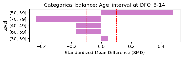
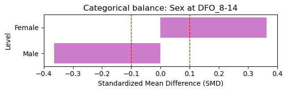
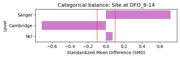
4.1 Baseline Covariate Balance (Treated vs Control)#
Here we assess baseline covariate balance between severity groups at the earliest visit. Standardized mean differences (SMD) below 0.1 indicate good balance.
[6]:
# Baseline covariate balance (select visit with most balanced counts)
covariates = [c for c in ["Age_interval", "Sex", "Site"] if c in adata.obs.columns]
if covariates:
    if "dfo_bin" in adata.obs.columns:
        # Pick visit with max min(n_treated, n_control) at participant-level
        visit_scores = []
        for v in sorted(adata.obs["dfo_bin"].dropna().unique()):
            sub = adata.obs[adata.obs["dfo_bin"] == v]
            if design.participant_col in sub.columns:
                counts = sub.groupby(design.arm_col)[design.participant_col].nunique()
            else:
                counts = sub.groupby(design.arm_col).size()
            n_t = int(counts.get(design.arm_treated, 0))
            n_c = int(counts.get(design.arm_control, 0))
            visit_scores.append((v, n_t, n_c, min(n_t, n_c)))
        # choose visit with largest min(n_t, n_c); tie-breaker by total participants
        visit_scores.sort(key=lambda x: (x[3], x[1]+x[2]), reverse=True)
        visit0, n_t, n_c, _ = visit_scores[0]
        print(f"Selected baseline visit: {visit0} (treated={n_t}, control={n_c})")

        try:
            balance = st.check_covariate_balance(adata, design, covariates, visit=visit0)
            if not balance.empty:
                # Numeric covariates: one figure
                num_bal = balance[balance["level"].isna()].copy()
                if not num_bal.empty:
                    plt.figure(figsize=(6, max(2, 0.4 * len(num_bal))))
                    sns.barplot(data=num_bal, y="covariate", x="smd", color="steelblue")
                    plt.axvline(0.1, color="red", linestyle="--", linewidth=1)
                    plt.axvline(-0.1, color="red", linestyle="--", linewidth=1)
                    plt.title(f"Numeric covariate balance at {visit0}")
                    plt.xlabel("Standardized Mean Difference (SMD)")
                    plt.ylabel("Covariate")
                    plt.tight_layout()
                    plt.show()

                # Categorical covariates: one panel per covariate
                cat_bal = balance[balance["level"].notna()].copy()
                for cov in cat_bal["covariate"].unique():
                    sub = cat_bal[cat_bal["covariate"] == cov].copy()
                    sub = sub.reindex(sub["smd"].abs().sort_values(ascending=False).index)
                    plt.figure(figsize=(6, max(2, 0.35 * len(sub))))
                    sns.barplot(data=sub, y="level", x="smd", color="orchid")
                    plt.axvline(0.1, color="red", linestyle="--", linewidth=1)
                    plt.axvline(-0.1, color="red", linestyle="--", linewidth=1)
                    plt.title(f"Categorical balance: {cov} at {visit0}")
                    plt.xlabel("Standardized Mean Difference (SMD)")
                    plt.ylabel("Level")
                    plt.tight_layout()
                    plt.show()
        except Exception as e:
            print(f"Covariate balance check failed: {e}")
    else:
        print("dfo_bin not found; skipping covariate balance check.")
else:
    print("No baseline covariates available for balance checking.")
Selected baseline visit: DFO_8-14 (treated=5, control=11)
[7]:
# Covariates for adjusted analyses (baseline balance indicated imbalance)
covariates_adj = [c for c in ["Age_interval", "Sex", "Site"] if c in adata.obs.columns]
print("Adjusted covariates:", covariates_adj)
Adjusted covariates: ['Age_interval', 'Sex', 'Site']
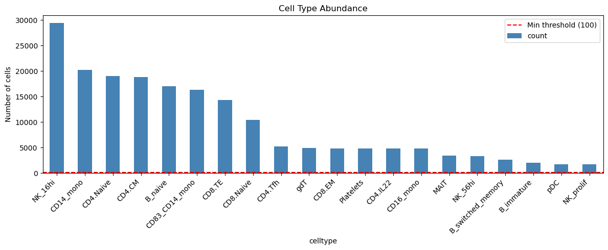
5. Cell Type Quality Control#
Filter to well-represented cell types for robust analysis.
[8]:
# Cell type counts
ct_counts = adata.obs["celltype"].value_counts()
print(f"Total cell types: {len(ct_counts)}")

# Filter to well-represented types
valid_celltypes = ct_counts[ct_counts >= MIN_CELLS_PER_CELLTYPE].index.tolist()
print(f"Cell types with ≥{MIN_CELLS_PER_CELLTYPE} cells: {len(valid_celltypes)}")

# Show top cell types
print("\nTop 15 cell types:")
display(ct_counts.head(15).to_frame("n_cells"))

# Visualize
fig, ax = plt.subplots(figsize=(12, 5))
ct_counts.head(20).plot(kind="bar", ax=ax, color="steelblue")
ax.axhline(MIN_CELLS_PER_CELLTYPE, color="red", linestyle="--", label=f"Min threshold ({MIN_CELLS_PER_CELLTYPE})")
ax.set_title("Cell Type Abundance")
ax.set_ylabel("Number of cells")
ax.legend()
plt.xticks(rotation=45, ha="right")
plt.tight_layout()
plt.show()
Total cell types: 50
Cell types with ≥100 cells: 41

Top 15 cell types:
| n_cells | |
|---|---|
| celltype | |
| NK_16hi | 29417 |
| CD14_mono | 20207 |
| CD4.Naive | 19076 |
| CD4.CM | 18804 |
| B_naive | 17063 |
| CD83_CD14_mono | 16326 |
| CD8.TE | 14366 |
| CD8.Naive | 10469 |
| CD4.Tfh | 5196 |
| gdT | 4938 |
| CD8.EM | 4864 |
| Platelets | 4824 |
| CD4.IL22 | 4817 |
| CD16_mono | 4790 |
| MAIT | 3475 |
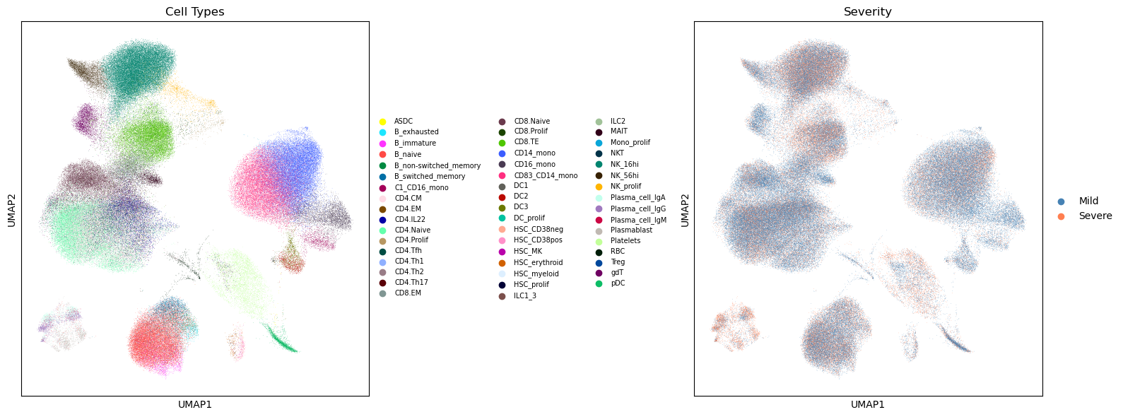
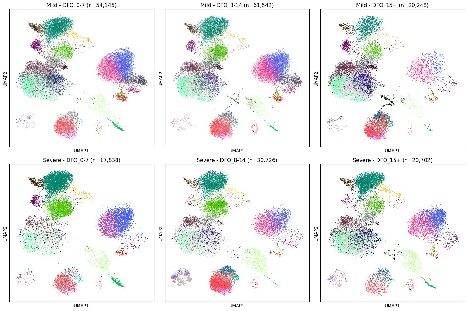
6. UMAP Visualization#
[9]:
# Compute UMAP if missing
if "X_umap" not in adata.obsm:
    print("Computing UMAP...")
    sc.pp.pca(adata)
    sc.pp.neighbors(adata)
    sc.tl.umap(adata)

# Global UMAP colored by cell type
fig, axes = plt.subplots(1, 2, figsize=(16, 6))

sc.pl.umap(adata, color="celltype", ax=axes[0], show=False,
           legend_loc="right margin", legend_fontsize=7, title="Cell Types")
sc.pl.umap(adata, color="severity", ax=axes[1], show=False,
           palette=["steelblue", "coral"], title="Severity")

plt.tight_layout()
plt.show()

# UMAP by severity and DFO
fig, axes = plt.subplots(2, 3, figsize=(15, 10))
for i, severity in enumerate(["Mild", "Severe"]):
    for j, dfo in enumerate(["DFO_0-7", "DFO_8-14", "DFO_15+"]):
        ax = axes[i, j]
        mask = (adata.obs["severity"] == severity) & (adata.obs["dfo_bin"] == dfo)
        if mask.sum() > 0:
            sub = adata[mask].copy()
            sc.pl.umap(sub, color="celltype", ax=ax, show=False,
                      legend_loc="none", title=f"{severity} - {dfo} (n={mask.sum():,})")
        else:
            ax.set_title(f"{severity} - {dfo} (no cells)")
            ax.axis("off")

plt.tight_layout()
plt.show()
7. COVID-19 Immune Signatures#
We define biologically relevant gene signatures for COVID-19 immune profiling, including:
Interferon response: Key antiviral pathway, often elevated in severe disease
Inflammation: S100 alarmins and cytokines associated with cytokine storm
Cytotoxicity: NK/CD8 T cell function, important for viral clearance
T cell exhaustion: Dysfunction markers elevated in severe/prolonged infection
Myeloid activation: Monocyte/macrophage markers, drivers of pathology
[10]:
available_genes = set(adata.var_names)

# COVID-19 relevant gene signatures
gene_signatures = {
    "IFN_Response": [
        "ISG15", "IFI6", "IFIT1", "IFIT2", "IFIT3", "MX1", "MX2",
        "STAT1", "STAT2", "OAS1", "OAS2", "OAS3", "IRF7", "IFITM1", "IFITM3"
    ],
    "Inflammation": [
        "S100A8", "S100A9", "S100A12", "LYZ", "VCAN", "IL1B",
        "CXCL8", "TNF", "NFKBIA", "CCL2", "CCL3", "CCL4"
    ],
    "Cytotoxicity": [
        "GZMB", "GZMA", "GZMH", "GZMK", "PRF1", "GNLY", "NKG7",
        "KLRD1", "KLRB1", "IFNG"
    ],
    "T_Cell_Exhaustion": [
        "PDCD1", "LAG3", "HAVCR2", "TIGIT", "CTLA4", "TOX", "ENTPD1"
    ],
    "Myeloid_Activation": [
        "CD14", "FCGR3A", "CD68", "MARCO", "MSR1", "CD163",
        "CTSS", "CST3", "LGALS3", "AIF1"
    ],
    "B_Cell_Activation": [
        "MS4A1", "CD19", "CD79A", "CD79B", "BANK1", "CD74",
        "HLA-DRA", "HLA-DRB1", "IGHM", "IGHG1"
    ],
}

# Filter to available genes and report coverage
print("Gene signature coverage:")
print("-" * 50)
filtered_signatures = {}
for name, genes in gene_signatures.items():
    found = [g for g in genes if g in available_genes]
    pct = len(found) / len(genes) * 100
    print(f"{name}: {len(found)}/{len(genes)} genes ({pct:.0f}%)")
    if len(found) >= MIN_GENES_FOR_SCORE:
        filtered_signatures[name] = found
    else:
        print(f"  ⚠️  Skipping (need ≥{MIN_GENES_FOR_SCORE} genes)")

# Score gene sets using z-mean method (accounts for different expression scales)
if filtered_signatures:
    adata = st.score_gene_sets(
        adata,
        filtered_signatures,
        layer="log1p_cpm",
        method="zmean",  # Z-score normalization for fair weighting
        prefix="sig_"
    )
    print(f"\n✓ Scored {len(filtered_signatures)} signatures")

# Get signature columns
signature_cols = [c for c in adata.obs.columns if c.startswith("sig_")]
print(f"\nSignature scores available: {signature_cols}")
Gene signature coverage:
--------------------------------------------------
IFN_Response: 15/15 genes (100%)
Inflammation: 12/12 genes (100%)
Cytotoxicity: 10/10 genes (100%)
T_Cell_Exhaustion: 7/7 genes (100%)
Myeloid_Activation: 10/10 genes (100%)
B_Cell_Activation: 10/10 genes (100%)

✓ Scored 6 signatures

Signature scores available: ['sig_IFN_Response', 'sig_Inflammation', 'sig_Cytotoxicity', 'sig_T_Cell_Exhaustion', 'sig_Myeloid_Activation', 'sig_B_Cell_Activation']
8. Cross-Sectional Comparisons: Severity Differences at Each Timepoint#
This is the primary analysis. We compare immune signatures between Mild and Severe patients at each DFO timepoint, using:
Participant-level aggregation (to avoid pseudoreplication)
Cell-type adjustment (to account for compositional differences)
FDR correction for multiple testing
[11]:
# Run comparisons at each timepoint using sctrial's built-in function
# This properly aggregates to participant level and handles the statistics correctly
print("="*60)
print("CROSS-SECTIONAL ANALYSIS: Severe vs Mild at each DFO bin")
print("="*60)
print("\nPositive beta = higher in Severe; Negative beta = higher in Mild")
print("Using participant-level aggregation to avoid pseudoreplication\n")

# Use a lower threshold (3) to include more timepoints for exploratory analysis
MIN_CROSS_SECTIONAL = 3

all_results = []
for visit in available_visits:
    print(f"\n{visit}:")

    # Check sample size first
    ad_visit = adata[adata.obs["dfo_bin"] == visit]
    n_per_group = ad_visit.obs.groupby("severity")["participant_id"].nunique()
    n_min = n_per_group.min()

    if n_min < MIN_CROSS_SECTIONAL:
        print(f"  Skipped: Insufficient participants (Mild={n_per_group.get('Mild', 0)}, Severe={n_per_group.get('Severe', 0)})")
        continue

    if n_min < MIN_PARTICIPANTS_FOR_COMPARISON:
        print(f"  Note: Small sample (Mild={n_per_group.get('Mild', 0)}, Severe={n_per_group.get('Severe', 0)}) — interpret with caution")

    # Use sctrial's built-in between_arm_comparison
    # This properly aggregates to participant level
    res = st.between_arm_comparison(
        adata,
        visit=visit,
        features=signature_cols,
        design=design,
        aggregate="participant_visit",
        standardize=True,
        method="ols",
    )

    if not res.empty:
        # Rename columns for consistency
        res = res.rename(columns={"beta_arm": "beta", "p_arm": "p_value", "FDR_arm": "fdr"})
        res["timepoint"] = visit
        all_results.append(res)

        # Display results
        display_cols = ["feature", "beta", "p_value", "fdr", "n_units"]
        display(res[display_cols].round(4))

        # Highlight significant
        sig = res[res["fdr"] < FDR_ALPHA]
        if not sig.empty:
            print(f"  Significant (FDR<{FDR_ALPHA}): {sig['feature'].tolist()}")

# Combine results
if all_results:
    combined_results = pd.concat(all_results, ignore_index=True)
else:
    combined_results = pd.DataFrame()
============================================================
CROSS-SECTIONAL ANALYSIS: Severe vs Mild at each DFO bin
============================================================

Positive beta = higher in Severe; Negative beta = higher in Mild
Using participant-level aggregation to avoid pseudoreplication


DFO_0-7:
  Skipped: Insufficient participants (Mild=8, Severe=2)

DFO_15+:
  Note: Small sample (Mild=4, Severe=4) — interpret with caution
| feature | beta | p_value | fdr | n_units | |
|---|---|---|---|---|---|
| 0 | sig_IFN_Response | 0.4732 | 0.5456 | 0.6547 | 8 |
| 1 | sig_Inflammation | 1.3433 | 0.0449 | 0.2692 | 8 |
| 2 | sig_Cytotoxicity | 0.6567 | 0.3939 | 0.6136 | 8 |
| 3 | sig_T_Cell_Exhaustion | 0.2095 | 0.7917 | 0.7917 | 8 |
| 4 | sig_Myeloid_Activation | 0.6372 | 0.4091 | 0.6136 | 8 |
| 5 | sig_B_Cell_Activation | -1.0558 | 0.1451 | 0.4352 | 8 |
DFO_8-14:
| feature | beta | p_value | fdr | n_units | |
|---|---|---|---|---|---|
| 0 | sig_IFN_Response | -0.0684 | 0.9042 | 0.9712 | 16 |
| 1 | sig_Inflammation | -0.0576 | 0.9192 | 0.9712 | 16 |
| 2 | sig_Cytotoxicity | 0.1428 | 0.8014 | 0.9712 | 16 |
| 3 | sig_T_Cell_Exhaustion | 0.7136 | 0.1953 | 0.5860 | 16 |
| 4 | sig_Myeloid_Activation | 0.0205 | 0.9712 | 0.9712 | 16 |
| 5 | sig_B_Cell_Activation | 1.0750 | 0.0414 | 0.2483 | 16 |
Significant (FDR<0.25): ['sig_B_Cell_Activation']
6.1 Adjusted Cross-Sectional Comparisons#
[12]:
# Adjusted cross-sectional analysis (includes covariates)
print('\nAdjusted cross-sectional analysis (covariates):', covariates_adj)
cross_sectional_adj = []
features_adj = signature_cols
visits_adj = tuple(sorted(
    adata.obs[design.visit_col].dropna().unique(),
    key=lambda c: int(c.split('_')[1].split('-')[0].rstrip('+')),
)[:2])
if features_adj:
    for v in visits_adj:
        print(f'\nAdjusted results at visit: {v}')
        res = st.between_arm_comparison(
            adata,
            visit=v,
            features=features_adj,
            design=design,
            aggregate='participant_visit',
            standardize=True,
            method='ols',
            covariates=covariates_adj if covariates_adj else None,
        )
        if res is not None and not res.empty:
            res['visit'] = v
            cross_sectional_adj.append(res)
            display(res[['feature', 'beta_arm', 'p_arm', 'FDR_arm', 'n_units']].round(4))
if cross_sectional_adj:
    all_cross_adj = __import__('pandas').concat(cross_sectional_adj, ignore_index=True)
else:
    all_cross_adj = __import__('pandas').DataFrame()
Adjusted cross-sectional analysis (covariates): ['Age_interval', 'Sex', 'Site']

Adjusted results at visit: DFO_0-7
| feature | beta_arm | p_arm | FDR_arm | n_units | |
|---|---|---|---|---|---|
| 0 | sig_IFN_Response | 0.0000 | 0.9999 | 0.9999 | 10 |
| 1 | sig_Inflammation | -0.6617 | 0.5035 | 0.7553 | 10 |
| 2 | sig_Cytotoxicity | 1.5344 | 0.3092 | 0.7016 | 10 |
| 3 | sig_T_Cell_Exhaustion | 0.0728 | 0.9344 | 0.9999 | 10 |
| 4 | sig_Myeloid_Activation | -0.8469 | 0.2063 | 0.7016 | 10 |
| 5 | sig_B_Cell_Activation | -1.4705 | 0.3508 | 0.7016 | 10 |
Adjusted results at visit: DFO_8-14
| feature | beta_arm | p_arm | FDR_arm | n_units | |
|---|---|---|---|---|---|
| 0 | sig_IFN_Response | -0.3551 | 0.4643 | 0.8604 | 16 |
| 1 | sig_Inflammation | 0.0796 | 0.8381 | 0.8604 | 16 |
| 2 | sig_Cytotoxicity | -0.1519 | 0.8604 | 0.8604 | 16 |
| 3 | sig_T_Cell_Exhaustion | 0.4013 | 0.5100 | 0.8604 | 16 |
| 4 | sig_Myeloid_Activation | 0.0866 | 0.8155 | 0.8604 | 16 |
| 5 | sig_B_Cell_Activation | 0.9085 | 0.2525 | 0.8604 | 16 |
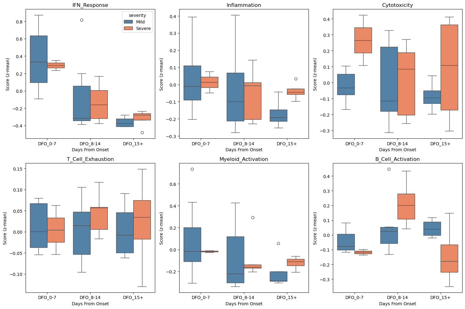
9. Visualization of Severity Differences#
[13]:
# Visualize signature distributions by severity and timepoint
fig, axes = plt.subplots(2, 3, figsize=(15, 10))
for i, sig in enumerate(signature_cols[:6]):
ax = axes.flat[i]
# Aggregate to participant level for cleaner visualization
df_plot = (
adata.obs
.groupby(["participant_id", "severity", "dfo_bin"], observed=True)[sig]
.mean()
.reset_index()
)
sns.boxplot(
data=df_plot, x="dfo_bin", y=sig, hue="severity",
palette={"Mild": "steelblue", "Severe": "coral"},
ax=ax
)
ax.set_title(sig.replace("sig_", ""))
ax.set_xlabel("Days From Onset")
ax.set_ylabel("Score (z-mean)")
if i > 0:
ax.get_legend().remove()
plt.tight_layout()
plt.show()
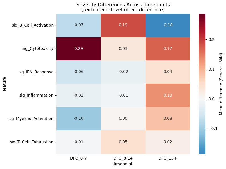
# Heatmap of effect sizes across ALL visits (computed directly from participant means)
# Uses a lower threshold (≥2 per group) for visualization purposes
heatmap_rows = []
for visit in available_visits:
ad_v = adata[adata.obs["dfo_bin"] == visit]
df_agg = (
ad_v.obs
.groupby(["participant_id", "severity"], observed=True)[signature_cols]
.mean()
.reset_index()
)
n_mild = (df_agg["severity"] == "Mild").sum()
n_severe = (df_agg["severity"] == "Severe").sum()
if min(n_mild, n_severe) < 2:
continue
for sig in signature_cols:
mild_vals = df_agg.loc[df_agg["severity"] == "Mild", sig].values
severe_vals = df_agg.loc[df_agg["severity"] == "Severe", sig].values
diff = severe_vals.mean() - mild_vals.mean()
heatmap_rows.append({"feature": sig, "timepoint": visit, "diff": diff})
if heatmap_rows:
df_heatmap = pd.DataFrame(heatmap_rows)
pivot = df_heatmap.pivot(index="feature", columns="timepoint", values="diff")
# Sort columns chronologically (alphabetical puts DFO_15-27 before DFO_8-14)
pivot = pivot[sorted(pivot.columns, key=lambda c: int(c.split("_")[1].split("-")[0].rstrip("+")))]
plt.figure(figsize=(8, 6))
sns.heatmap(
pivot, cmap="RdBu_r", center=0, annot=True, fmt=".2f",
cbar_kws={"label": "Mean difference (Severe - Mild)"}
)
plt.title("Severity Differences Across Timepoints\n(participant-level mean difference)")
plt.tight_layout()
plt.show()
elif not combined_results.empty:
pivot = combined_results.pivot(index="feature", columns="timepoint", values="beta")
pivot = pivot[sorted(pivot.columns, key=lambda c: int(c.split("_")[1].split("-")[0].rstrip("+")))]
plt.figure(figsize=(8, 6))
sns.heatmap(
pivot, cmap="RdBu_r", center=0, annot=True, fmt=".2f",
cbar_kws={"label": "Effect size (Severe - Mild)"}
)
plt.title("Severity Effect Sizes Across Timepoints")
plt.tight_layout()
plt.show()
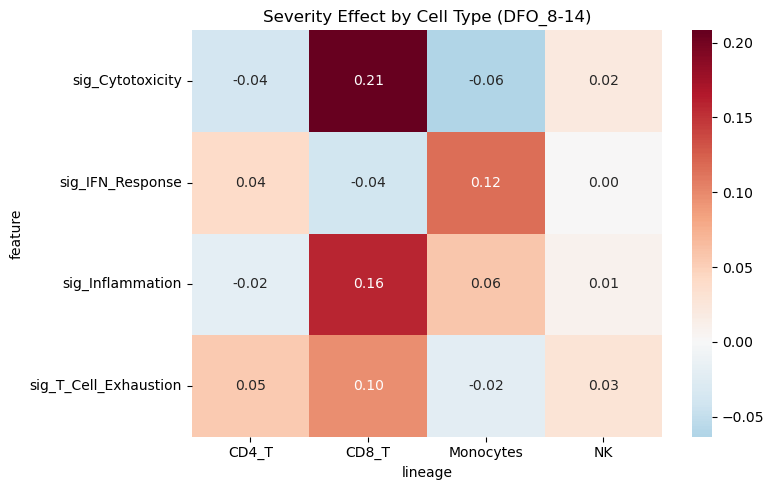
10. Cell-Type Specific Analysis#
Examine severity differences within specific immune cell populations.
[14]:
# Focus on major immune populations
# Map fine cell types to major lineages for robust analysis
adata.obs["lineage"] = adata.obs["celltype"].apply(categorize_celltype)
print("Lineage distribution:")
print(adata.obs["lineage"].value_counts())

focus_lineages = ["CD4_T", "CD8_T", "Monocytes", "NK"]

# Auto-select the visit with the best participant balance across arms
visit_scores = []
for v in sorted(adata.obs["dfo_bin"].dropna().unique()):
    sub = adata.obs[adata.obs["dfo_bin"] == v]
    counts = sub.groupby("severity")["participant_id"].nunique()
    n_mild = int(counts.get("Mild", 0))
    n_severe = int(counts.get("Severe", 0))
    visit_scores.append((v, n_mild, n_severe, min(n_mild, n_severe)))
visit_scores.sort(key=lambda x: (x[3], x[1] + x[2]), reverse=True)
focus_visit = visit_scores[0][0]

print(f"\n=== Cell-Type Specific Analysis at {focus_visit} ===")
print(f"    (auto-selected: best participant balance across arms)")

# Use sctrial between_arm_comparison per lineage
lineage_results = []
for lineage in focus_lineages:
    ad_sub = adata[(adata.obs["lineage"] == lineage) & (adata.obs["dfo_bin"] == focus_visit)].copy()
    if ad_sub.n_obs < 100:
        print(f"{lineage}: Insufficient cells ({ad_sub.n_obs})")
        continue
    n_per_group = ad_sub.obs.groupby("severity")["participant_id"].nunique()
    if n_per_group.min() < 3:
        print(f"{lineage}: Insufficient participants")
        continue
    print(f"{lineage} (n={ad_sub.n_obs:,} cells, {n_per_group.sum()} participants):")

    res = st.between_arm_comparison(
        ad_sub,
        visit=focus_visit,
        features=signature_cols[:4],
        design=design,
        method="wilcoxon",
    )
    res["lineage"] = lineage
    lineage_results.append(res)

if lineage_results:
    df_lineage = pd.concat(lineage_results, ignore_index=True)
    # Add FDR correction across all tests
    from statsmodels.stats.multitest import multipletests
    df_lineage["FDR"] = multipletests(df_lineage["p_arm"], method="fdr_bh")[1]
    print("\nResults (participant-level Mann-Whitney U via sctrial):")
    display(df_lineage[["lineage", "feature", "beta_arm", "p_arm", "FDR"]].round(4))

    # Pivot for heatmap
    pivot = df_lineage.pivot(index="feature", columns="lineage", values="beta_arm")
    plt.figure(figsize=(8, 5))
    sns.heatmap(pivot, cmap="RdBu_r", center=0, annot=True, fmt=".2f")
    plt.title(f"Severity Effect by Cell Type ({focus_visit})")
    plt.tight_layout()
    plt.show()
Lineage distribution:
lineage
CD4_T        49451
CD8_T        46464
Other        38546
NK           35643
Monocytes    26237
B_cells       4827
DCs           4034
Name: count, dtype: int64

=== Cell-Type Specific Analysis at DFO_8-14 ===
    (auto-selected: best participant balance across arms)
CD4_T (n=20,684 cells, 16 participants):
CD8_T (n=22,232 cells, 16 participants):
Monocytes (n=11,322 cells, 15 participants):
NK (n=14,538 cells, 16 participants):

Results (participant-level Mann-Whitney U via sctrial):
| lineage | feature | beta_arm | p_arm | FDR | |
|---|---|---|---|---|---|
| 0 | CD4_T | sig_IFN_Response | 0.0404 | 0.9130 | 1.0000 |
| 1 | CD4_T | sig_Inflammation | -0.0197 | 0.9130 | 1.0000 |
| 2 | CD4_T | sig_Cytotoxicity | -0.0369 | 0.5833 | 1.0000 |
| 3 | CD4_T | sig_T_Cell_Exhaustion | 0.0545 | 0.0897 | 0.9194 |
| 4 | CD8_T | sig_IFN_Response | -0.0394 | 1.0000 | 1.0000 |
| 5 | CD8_T | sig_Inflammation | 0.1593 | 0.6612 | 1.0000 |
| 6 | CD8_T | sig_Cytotoxicity | 0.2083 | 0.2212 | 1.0000 |
| 7 | CD8_T | sig_T_Cell_Exhaustion | 0.0961 | 0.1149 | 0.9194 |
| 8 | Monocytes | sig_IFN_Response | 0.1161 | 0.8591 | 1.0000 |
| 9 | Monocytes | sig_Inflammation | 0.0580 | 0.5135 | 1.0000 |
| 10 | Monocytes | sig_Cytotoxicity | -0.0634 | 0.8591 | 1.0000 |
| 11 | Monocytes | sig_T_Cell_Exhaustion | -0.0218 | 0.9530 | 1.0000 |
| 12 | NK | sig_IFN_Response | 0.0015 | 1.0000 | 1.0000 |
| 13 | NK | sig_Inflammation | 0.0093 | 0.9130 | 1.0000 |
| 14 | NK | sig_Cytotoxicity | 0.0206 | 0.6612 | 1.0000 |
| 15 | NK | sig_T_Cell_Exhaustion | 0.0294 | 0.6612 | 1.0000 |
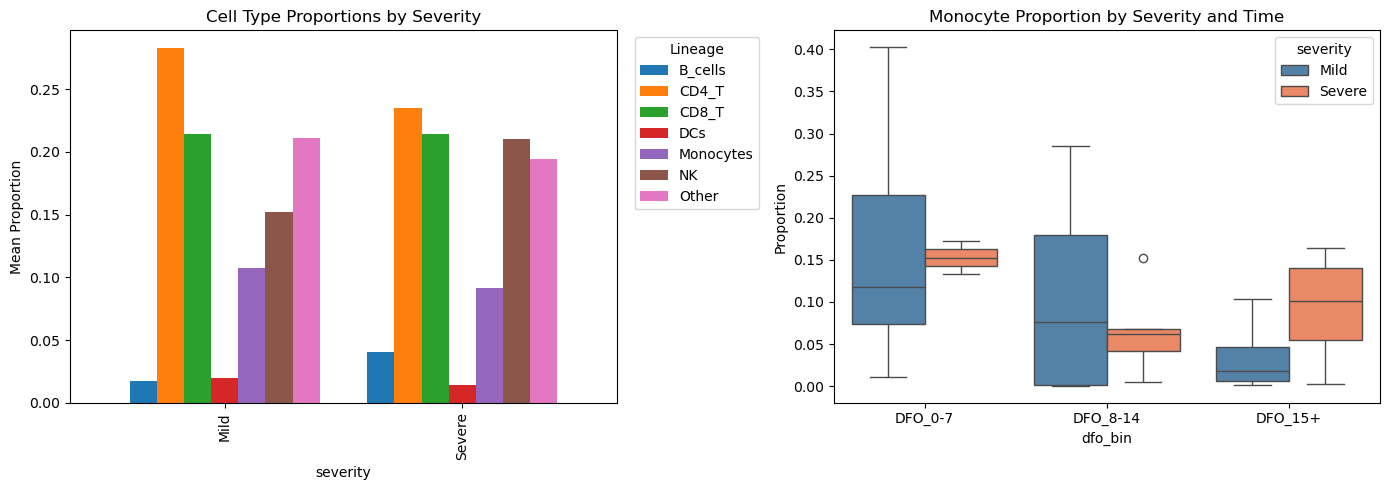
11. Cell Type Abundance Differences#
Compare cell type composition between severity groups.
[15]:
# Calculate cell type proportions per participant
# Note: Each row in 'props' after grouping is one participant-visit-lineage combination
# When we test, each participant contributes ONE proportion value per lineage
props = (
    adata.obs
    .groupby(["participant_id", "severity", "dfo_bin", "lineage"], observed=True)
    .size()
    .reset_index(name="n")
)
totals = props.groupby(["participant_id", "dfo_bin"])["n"].transform("sum")
props["proportion"] = props["n"] / totals

# Visualize
fig, axes = plt.subplots(1, 2, figsize=(14, 5))

# By severity
props_by_sev = props.groupby(["severity", "lineage"])["proportion"].mean().unstack()
props_by_sev.plot(kind="bar", ax=axes[0], width=0.8)
axes[0].set_title("Cell Type Proportions by Severity")
axes[0].set_ylabel("Mean Proportion")
axes[0].legend(title="Lineage", bbox_to_anchor=(1.02, 1))

# Monocyte proportion over time
mono_props = props[props["lineage"] == "Monocytes"].copy()
sns.boxplot(data=mono_props, x="dfo_bin", y="proportion", hue="severity",
            palette={"Mild": "steelblue", "Severe": "coral"}, ax=axes[1])
axes[1].set_title("Monocyte Proportion by Severity and Time")
axes[1].set_ylabel("Proportion")

plt.tight_layout()
plt.show()

# Statistical test for abundance differences
# CORRECT: Each observation in props_early is already at participant level
# so Mann-Whitney U is appropriate here (no pseudoreplication)
print("\nAbundance differences (Severe vs Mild) at DFO 0-7:")
print("Note: Each data point = one participant's cell type proportion")
print("-" * 50)

props_early = props[props["dfo_bin"] == "DFO_0-7"]
abundance_results = []
for lineage in ["Monocytes", "CD8_T", "NK", "B_cells"]:
    sub = props_early[props_early["lineage"] == lineage]
    mild = sub.loc[sub["severity"] == "Mild", "proportion"]
    severe = sub.loc[sub["severity"] == "Severe", "proportion"]

    if len(mild) >= 3 and len(severe) >= 3:
        stat, pval = mannwhitneyu(mild, severe, alternative="two-sided")
        diff = severe.mean() - mild.mean()
        abundance_results.append({
            "lineage": lineage,
            "diff": diff,
            "p_value": pval,
            "n_mild": len(mild),
            "n_severe": len(severe),
        })
        print(f"{lineage}: diff={diff:+.3f}, p={pval:.4f} (n_mild={len(mild)}, n_severe={len(severe)})")

if abundance_results:
    df_abund = pd.DataFrame(abundance_results)
    df_abund["fdr"] = multipletests(df_abund["p_value"], method="fdr_bh")[1]
    print(f"\nFDR-corrected results:")
    display(df_abund.round(4))
Abundance differences (Severe vs Mild) at DFO 0-7:
Note: Each data point = one participant's cell type proportion
--------------------------------------------------
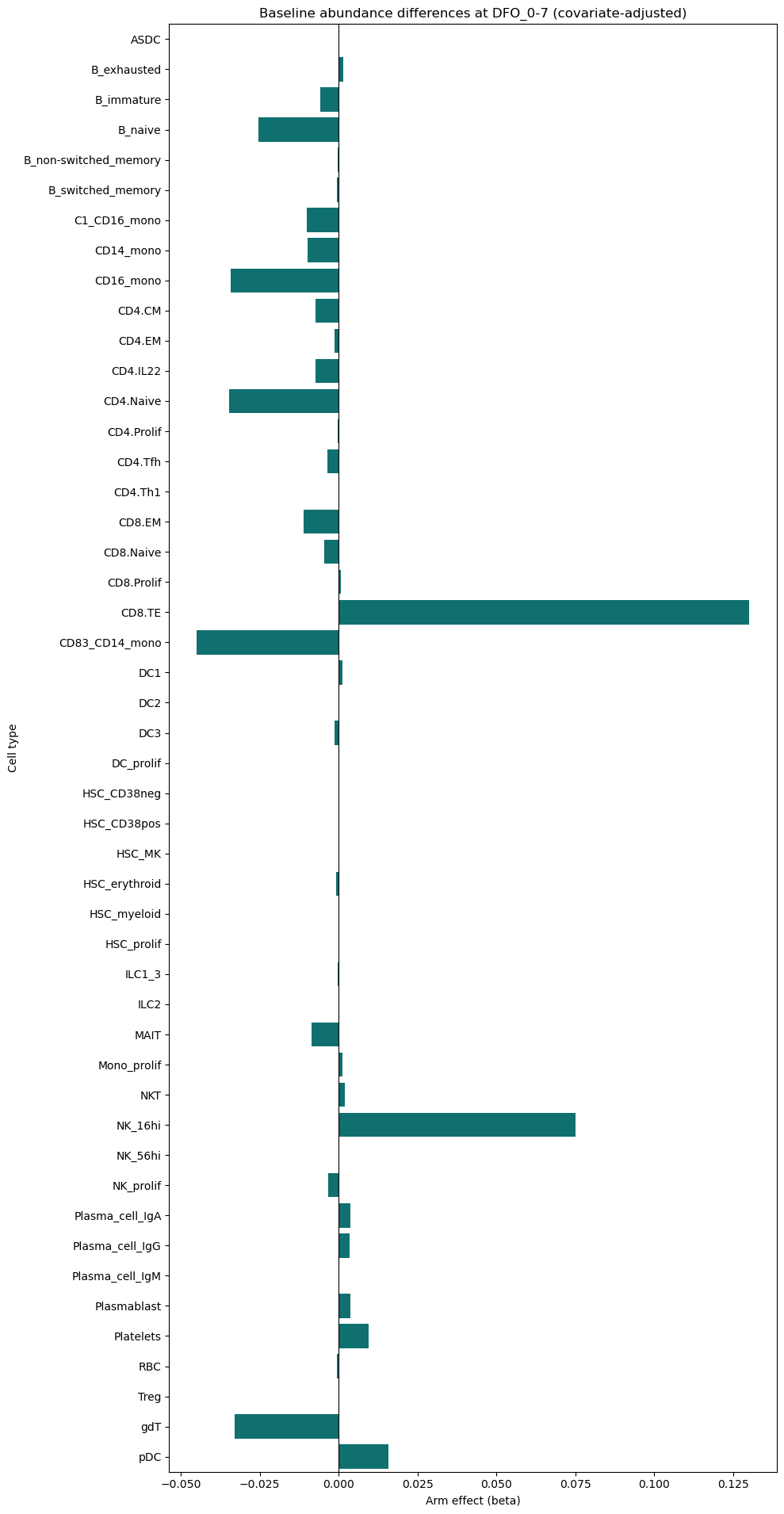
9.1 Adjusted Abundance DiD#
[16]:
# Adjusted abundance DiD (covariates)
print('\nAdjusted abundance DiD (covariates):', covariates_adj)
# Build numeric covariates for abundance models when possible
covariates_ab = []
if 'Age_interval' in adata.obs.columns:
    # Convert intervals like '(50, 59]' to midpoint
    def _age_mid(x):
        try:
            s = str(x).strip().strip('()[]')
            lo, hi = s.split(',')
            return (float(lo) + float(hi)) / 2
        except Exception:
            return float('nan')
    adata.obs['age_mid'] = adata.obs['Age_interval'].map(_age_mid)
    if adata.obs['age_mid'].notna().any():
        covariates_ab.append('age_mid')
if 'Sex' in adata.obs.columns:
    covariates_ab.append('Sex')
if 'Site' in adata.obs.columns:
    # high-cardinality sites can destabilize models; include only if <=3 levels
    if adata.obs['Site'].nunique() <= 3:
        covariates_ab.append('Site')
print('Adjusted abundance covariates:', covariates_ab)

if design.celltype_col:
    # Diagnostic: participant counts per celltype at selected visits
    visits_ab = sorted(
        adata.obs[design.visit_col].dropna().unique(),
        key=lambda c: int(c.split('_')[1].split('-')[0].rstrip('+')),
    )[:2]
    diag = (
        adata.obs[adata.obs[design.visit_col].isin(visits_ab)]
        .groupby([design.celltype_col, design.arm_col])[design.participant_col]
        .nunique()
        .unstack(fill_value=0)
    )
    print('Participant counts per cell type (treated/control):')
    display(diag)

    def _run_ab(covs, label):
        print(f'Attempt: {label} covariates -> {covs}')
        return st.abundance_did(
            adata,
            design,
            visits=tuple(visits_ab),
            covariates=covs if covs else None,
            min_units=3,
            use_bootstrap=True,
            n_boot=199,
            seed=SEED,
        )

    ab_adj = _run_ab(covariates_ab, 'full')
    if ab_adj is None or ab_adj.empty:
        # retry with numeric-only covariates
        num_covs = [c for c in covariates_ab if c == 'age_mid']
        ab_adj = _run_ab(num_covs, 'numeric-only')
    if ab_adj is None or ab_adj.empty:
        # final fallback: unadjusted
        ab_adj = _run_ab([], 'unadjusted fallback')

    if ab_adj is not None and not ab_adj.empty:
        display(ab_adj.round(4))
        try:
            plt.figure(figsize=(10, max(3, 0.4 * len(ab_adj))))
            sns.barplot(data=ab_adj, y='celltype', x='beta_DiD', color='teal')
            plt.axvline(0, color='black', linewidth=0.8)
            plt.title('Adjusted Abundance DiD (covariates)')
            plt.xlabel('DiD effect (beta)')
            plt.ylabel('Cell type')
            plt.tight_layout()
            plt.show()
        except Exception as e:
            print(f'Adjusted abundance plot failed: {e}')
    else:
        print('No adjusted abundance DiD results after retries.')


    # If DiD is not feasible (no paired participants), run cross-sectional abundance at baseline
    if ab_adj is None or ab_adj.empty:
        # Check paired participants overall
        visits_use = tuple(visits_ab)
        obs_use = adata.obs[adata.obs[design.visit_col].isin(visits_use)].copy()
        totals_all = (
            obs_use.groupby([design.participant_col, design.visit_col, design.arm_col], observed=True)
            .size()
            .reset_index(name='n_cells')
        )
        wide_tot = totals_all.pivot_table(
            index=design.participant_col,
            columns=design.visit_col,
            values='n_cells',
            aggfunc='mean',
            observed=True,
        )
        paired_units = wide_tot[wide_tot[visits_use[0]].notna() & wide_tot[visits_use[1]].notna()].index
        if len(paired_units) == 0:
            print('No paired participants for abundance DiD. Running baseline cross-sectional abundance instead.')
            baseline_visit = visits_use[0]
            obs_base = adata.obs[adata.obs[design.visit_col] == baseline_visit].copy()
            # proportions per participant × celltype
            counts_base = (
                obs_base.groupby([design.participant_col, design.arm_col, design.celltype_col], observed=True)
                .size()
                .reset_index(name='n_cells')
            )
            totals_base = (
                counts_base.groupby([design.participant_col, design.arm_col], observed=True)['n_cells']
                .sum()
                .reset_index(name='total_cells')
            )
            counts_base = counts_base.merge(totals_base, on=[design.participant_col, design.arm_col], how='left')
            counts_base['prop'] = counts_base['n_cells'] / counts_base['total_cells'].clip(lower=1)

            # attach covariates (participant-level)
            cov_df = obs_base[[design.participant_col] + covariates_ab].drop_duplicates()
            counts_base = counts_base.merge(cov_df, on=design.participant_col, how='left')
            counts_base['arm_bin'] = design.arm_bin(counts_base)
            counts_base = counts_base.dropna(subset=['arm_bin'])

            rows = []
            for ct in sorted(counts_base[design.celltype_col].unique()):
                tmp = counts_base[counts_base[design.celltype_col] == ct].copy()
                if tmp[design.participant_col].nunique() < 3:
                    continue
                if tmp['prop'].nunique() < 2:
                    continue
                formula = 'prop ~ arm_bin'
                if covariates_ab:
                    formula += ' + ' + ' + '.join(covariates_ab)
                import statsmodels.formula.api as smf
                fit = smf.ols(formula, data=tmp).fit()
                if 'arm_bin' not in fit.params or fit.params['arm_bin'] is None:
                    continue
                rows.append({
                    'celltype': ct,
                    'n_participants': int(tmp[design.participant_col].nunique()),
                    'beta_arm': float(fit.params['arm_bin']),
                    'p_arm': float(fit.pvalues['arm_bin']),
                })
            if rows:
                import pandas as pd
                from statsmodels.stats.multitest import multipletests
                res_xs = pd.DataFrame(rows)
                mask = res_xs['p_arm'].notna()
                res_xs['FDR_arm'] = pd.NA
                if mask.any():
                    res_xs.loc[mask, 'FDR_arm'] = multipletests(res_xs.loc[mask,'p_arm'], method='fdr_bh')[1]
                display(res_xs.sort_values('p_arm').head(20))
                try:
                    plt.figure(figsize=(10, max(3, 0.4 * len(res_xs))))
                    sns.barplot(data=res_xs, y='celltype', x='beta_arm', color='teal')
                    plt.axvline(0, color='black', linewidth=0.8)
                    plt.title(f'Baseline abundance differences at {baseline_visit} (covariate-adjusted)')
                    plt.xlabel('Arm effect (beta)')
                    plt.ylabel('Cell type')
                    plt.tight_layout()
                    plt.show()
                except Exception as e:
                    print(f'Baseline abundance plot failed: {e}')
Adjusted abundance DiD (covariates): ['Age_interval', 'Sex', 'Site']
Adjusted abundance covariates: ['age_mid', 'Sex', 'Site']
Participant counts per cell type (treated/control):
| severity | Mild | Severe |
|---|---|---|
| celltype | ||
| ASDC | 13 | 4 |
| B_exhausted | 19 | 7 |
| B_immature | 19 | 7 |
| B_naive | 19 | 7 |
| B_non-switched_memory | 19 | 7 |
| B_switched_memory | 19 | 7 |
| C1_CD16_mono | 11 | 5 |
| CD4.CM | 19 | 7 |
| CD4.EM | 19 | 7 |
| CD4.IL22 | 19 | 7 |
| CD4.Naive | 19 | 7 |
| CD4.Prolif | 16 | 7 |
| CD4.Tfh | 19 | 7 |
| CD4.Th1 | 16 | 4 |
| CD4.Th2 | 5 | 3 |
| CD4.Th17 | 2 | 2 |
| CD8.EM | 19 | 7 |
| CD8.Naive | 19 | 7 |
| CD8.Prolif | 18 | 6 |
| CD8.TE | 19 | 7 |
| CD14_mono | 18 | 7 |
| CD16_mono | 16 | 7 |
| CD83_CD14_mono | 19 | 7 |
| DC1 | 15 | 4 |
| DC2 | 18 | 7 |
| DC3 | 19 | 7 |
| DC_prolif | 6 | 2 |
| HSC_CD38neg | 11 | 7 |
| HSC_CD38pos | 18 | 5 |
| HSC_MK | 4 | 4 |
| HSC_erythroid | 15 | 7 |
| HSC_myeloid | 6 | 3 |
| HSC_prolif | 7 | 2 |
| ILC1_3 | 15 | 7 |
| ILC2 | 7 | 2 |
| MAIT | 19 | 7 |
| Mono_prolif | 9 | 5 |
| NKT | 19 | 7 |
| NK_16hi | 19 | 7 |
| NK_56hi | 19 | 7 |
| NK_prolif | 19 | 7 |
| Plasma_cell_IgA | 18 | 7 |
| Plasma_cell_IgG | 19 | 7 |
| Plasma_cell_IgM | 17 | 7 |
| Plasmablast | 19 | 7 |
| Platelets | 19 | 7 |
| RBC | 13 | 7 |
| Treg | 11 | 3 |
| gdT | 19 | 7 |
| pDC | 18 | 7 |
Attempt: full covariates -> ['age_mid', 'Sex', 'Site']
Attempt: numeric-only covariates -> ['age_mid']
Attempt: unadjusted fallback covariates -> []
No adjusted abundance DiD results after retries.
No paired participants for abundance DiD. Running baseline cross-sectional abundance instead.
| celltype | n_participants | beta_arm | p_arm | FDR_arm | |
|---|---|---|---|---|---|
| 21 | DC1 | 7 | 0.001090 | 0.032445 | 0.781814 |
| 11 | CD4.IL22 | 10 | -0.007421 | 0.044069 | 0.781814 |
| 36 | NK_16hi | 10 | 0.075020 | 0.055844 | 0.781814 |
| 23 | DC3 | 10 | -0.001242 | 0.143460 | 0.875708 |
| 35 | NKT | 10 | 0.002001 | 0.147275 | 0.875708 |
| 19 | CD8.TE | 10 | 0.130125 | 0.165944 | 0.875708 |
| 2 | B_immature | 10 | -0.005815 | 0.167006 | 0.875708 |
| 1 | B_exhausted | 10 | 0.001560 | 0.173708 | 0.875708 |
| 28 | HSC_erythroid | 9 | -0.000836 | 0.218194 | 0.875708 |
| 6 | C1_CD16_mono | 8 | -0.010052 | 0.234704 | 0.875708 |
| 46 | gdT | 10 | -0.033003 | 0.295915 | 0.875708 |
| 47 | pDC | 10 | 0.015888 | 0.312960 | 0.875708 |
| 8 | CD16_mono | 10 | -0.034212 | 0.324744 | 0.875708 |
| 12 | CD4.Naive | 10 | -0.034840 | 0.337689 | 0.875708 |
| 42 | Plasmablast | 10 | 0.003829 | 0.337901 | 0.875708 |
| 39 | Plasma_cell_IgA | 10 | 0.003787 | 0.340136 | 0.875708 |
| 3 | B_naive | 10 | -0.025556 | 0.354453 | 0.875708 |
| 16 | CD8.EM | 10 | -0.011124 | 0.413749 | 0.909467 |
| 40 | Plasma_cell_IgG | 10 | 0.003477 | 0.427501 | 0.909467 |
| 34 | Mono_prolif | 6 | 0.001219 | 0.434371 | 0.909467 |
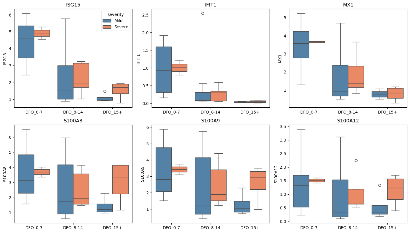
12. Individual Gene Analysis#
Examine specific genes of interest for COVID-19.
[17]:
# Key COVID-19 genes
covid_genes = [
"ISG15", "IFIT1", "MX1", # IFN response
"S100A8", "S100A9", "S100A12", # Alarmins
"GZMB", "PRF1", "NKG7", # Cytotoxicity
"IL1B", "TNF", "CXCL8", # Cytokines
]
covid_genes = [g for g in covid_genes if g in adata.var_names]
print(f"Analyzing {len(covid_genes)} COVID-relevant genes")
# Extract expression for visualization
gene_expr = pd.DataFrame(
adata[:, covid_genes].layers["log1p_cpm"].toarray() if sp.issparse(adata[:, covid_genes].layers["log1p_cpm"])
else adata[:, covid_genes].layers["log1p_cpm"],
columns=covid_genes,
index=adata.obs_names
)
gene_expr = gene_expr.join(adata.obs[["severity", "dfo_bin", "participant_id", "lineage"]])
# Aggregate to participant level
gene_means = gene_expr.groupby(["participant_id", "severity", "dfo_bin"])[covid_genes].mean().reset_index()
# Visualize key genes
fig, axes = plt.subplots(2, 3, figsize=(14, 8))
for i, gene in enumerate(covid_genes[:6]):
ax = axes.flat[i]
sns.boxplot(
data=gene_means, x="dfo_bin", y=gene, hue="severity",
palette={"Mild": "steelblue", "Severe": "coral"}, ax=ax
)
ax.set_title(gene)
ax.set_xlabel("")
if i > 0:
ax.get_legend().remove()
plt.tight_layout()
plt.show()
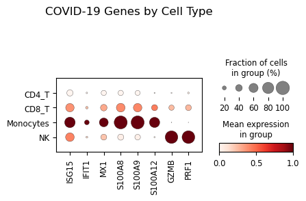
# Dotplot of genes by cell type
if len(covid_genes) > 0:
adata_dot = adata[adata.obs["lineage"].isin(["Monocytes", "CD8_T", "NK", "CD4_T"])].copy()
sc.pl.dotplot(
adata_dot,
var_names=covid_genes[:8],
groupby="lineage",
standard_scale="var",
title="COVID-19 Genes by Cell Type"
)
Analyzing 12 COVID-relevant genes
13. Advanced Statistical Analyses#
Statistical tools for cross-sectional observational data:
Effect sizes: Cohen’s d for severity group comparisons
Power analysis: Sample size planning for future studies
Effective sample size: Understanding clustering effects
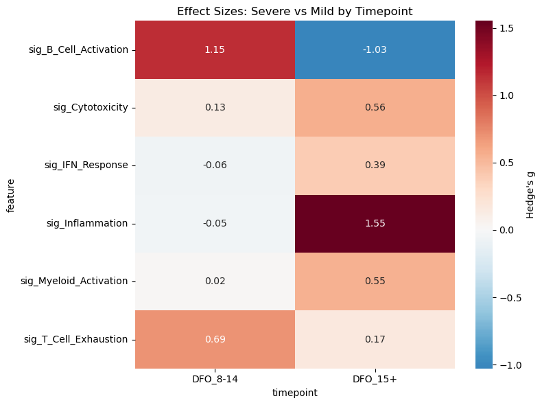
13.1 Effect Sizes for Cross-Sectional Comparisons#
Effect sizes quantify the magnitude of differences between Mild and Severe cases.
[18]:
print("=" * 60)
print("EFFECT SIZE ANALYSIS (Cross-Sectional)")
print("=" * 60)
if signature_cols:
# Calculate effect sizes for severity comparison at each timepoint
effect_results = []
for visit in available_visits:
ad_visit = adata[adata.obs["dfo_bin"] == visit]
# Aggregate to participant level
df_agg = (
ad_visit.obs
.groupby(["participant_id", "severity"], observed=True)[signature_cols]
.mean()
.reset_index()
)
for sig in signature_cols:
mild_vals = df_agg.loc[df_agg["severity"] == "Mild", sig].dropna().values
severe_vals = df_agg.loc[df_agg["severity"] == "Severe", sig].dropna().values
if len(mild_vals) >= 3 and len(severe_vals) >= 3:
# Cohen's d and Hedge's g
d = st.cohens_d(severe_vals, mild_vals) # Positive = higher in Severe
g = st.hedges_g(severe_vals, mild_vals)
# Bootstrap CI (returns: effect_size, ci_lower, ci_upper)
try:
_, ci_low, ci_high = st.bootstrap_effect_size_ci(
severe_vals, mild_vals,
n_boot=999,
alpha=0.05,
seed=SEED
)
except Exception:
ci_low, ci_high = np.nan, np.nan
effect_results.append({
"timepoint": visit,
"feature": sig,
"cohens_d": d,
"hedges_g": g,
"ci_lower": ci_low,
"ci_upper": ci_high,
"n_mild": len(mild_vals),
"n_severe": len(severe_vals),
})
if effect_results:
df_effect = pd.DataFrame(effect_results)
print("\nEffect sizes (Severe vs Mild):")
print(" Positive = higher in Severe, Negative = higher in Mild")
print("")
display(df_effect.round(3))
# Heatmap of effect sizes
pivot = df_effect.pivot(index="feature", columns="timepoint", values="hedges_g")
# Sort columns chronologically
pivot = pivot[sorted(pivot.columns, key=lambda c: int(c.split("_")[1].split("-")[0].rstrip("+")))]
plt.figure(figsize=(8, 6))
sns.heatmap(
pivot, cmap="RdBu_r", center=0, annot=True, fmt=".2f",
cbar_kws={"label": "Hedge's g"}
)
plt.title("Effect Sizes: Severe vs Mild by Timepoint")
plt.tight_layout()
plt.show()
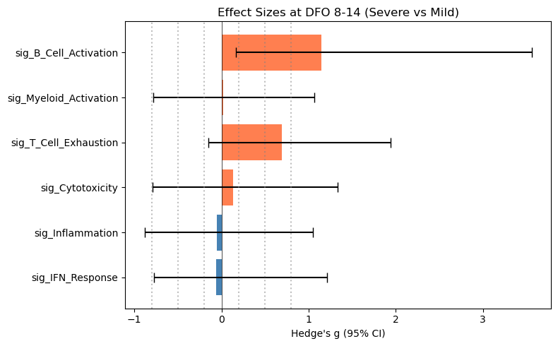
# Forest plot for one timepoint
visit_data = df_effect[df_effect["timepoint"] == "DFO_8-14"]
if not visit_data.empty:
fig, ax = plt.subplots(figsize=(8, 5))
y_pos = np.arange(len(visit_data))
ax.barh(y_pos, visit_data["hedges_g"], xerr=[
visit_data["hedges_g"] - visit_data["ci_lower"],
visit_data["ci_upper"] - visit_data["hedges_g"]
], capsize=5, color=["coral" if g > 0 else "steelblue" for g in visit_data["hedges_g"]])
ax.axvline(0, color="black", linewidth=0.5)
ax.set_yticks(y_pos)
ax.set_yticklabels(visit_data["feature"])
ax.set_xlabel("Hedge's g (95% CI)")
ax.set_title("Effect Sizes at DFO 8-14 (Severe vs Mild)")
# Reference lines
for thresh in [-0.8, -0.5, -0.2, 0.2, 0.5, 0.8]:
ax.axvline(thresh, color="gray", linestyle=":", alpha=0.5)
plt.tight_layout()
plt.show()
else:
print("No signature columns for effect size analysis.")
============================================================
EFFECT SIZE ANALYSIS (Cross-Sectional)
============================================================

Effect sizes (Severe vs Mild):
  Positive = higher in Severe, Negative = higher in Mild
| timepoint | feature | cohens_d | hedges_g | ci_lower | ci_upper | n_mild | n_severe | |
|---|---|---|---|---|---|---|---|---|
| 0 | DFO_15+ | sig_IFN_Response | 0.453 | 0.393 | -0.730 | 4.212 | 4 | 4 |
| 1 | DFO_15+ | sig_Inflammation | 1.787 | 1.552 | 0.527 | 5.782 | 4 | 4 |
| 2 | DFO_15+ | sig_Cytotoxicity | 0.649 | 0.564 | -1.608 | 5.717 | 4 | 4 |
| 3 | DFO_15+ | sig_T_Cell_Exhaustion | 0.195 | 0.170 | -1.177 | 2.273 | 4 | 4 |
| 4 | DFO_15+ | sig_Myeloid_Activation | 0.627 | 0.545 | -0.630 | 12.730 | 4 | 4 |
| 5 | DFO_15+ | sig_B_Cell_Activation | -1.184 | -1.028 | -4.996 | 0.038 | 4 | 4 |
| 6 | DFO_8-14 | sig_IFN_Response | -0.066 | -0.063 | -0.772 | 1.212 | 11 | 5 |
| 7 | DFO_8-14 | sig_Inflammation | -0.056 | -0.053 | -0.884 | 1.050 | 11 | 5 |
| 8 | DFO_8-14 | sig_Cytotoxicity | 0.138 | 0.131 | -0.791 | 1.333 | 11 | 5 |
| 9 | DFO_8-14 | sig_T_Cell_Exhaustion | 0.734 | 0.693 | -0.150 | 1.941 | 11 | 5 |
| 10 | DFO_8-14 | sig_Myeloid_Activation | 0.020 | 0.019 | -0.785 | 1.062 | 11 | 5 |
| 11 | DFO_8-14 | sig_B_Cell_Activation | 1.211 | 1.145 | 0.164 | 3.557 | 11 | 5 |
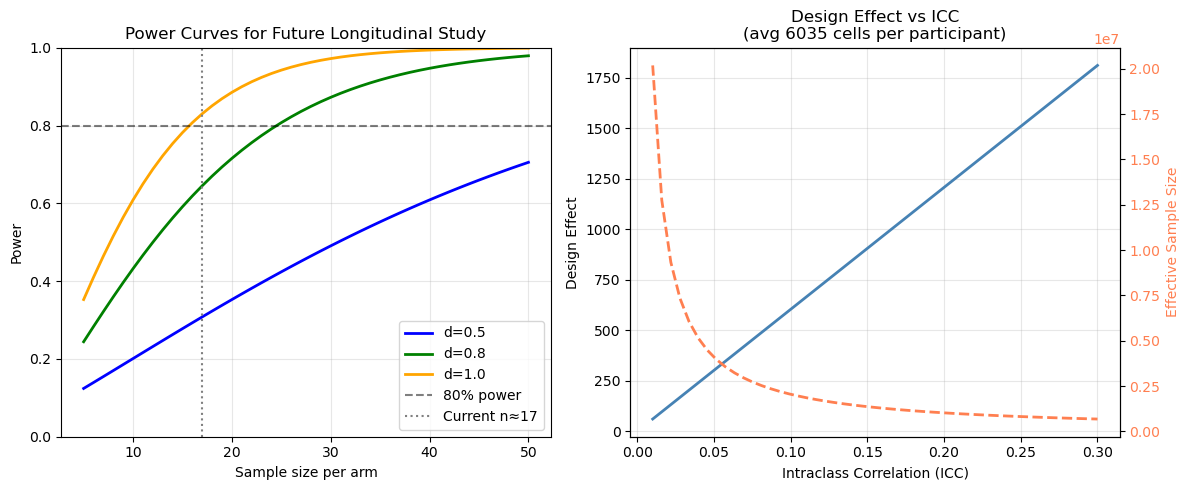
13.2 Power Analysis#
Power analysis helps understand what effect sizes this study could detect and plan future longitudinal studies.
Caveat: This dataset has no longitudinally paired participants for the primary Mild vs Severe comparison. The power curves below use the average group size as a rough guide for what a future paired longitudinal study of this scale could detect — they do not represent the power of the current cross-sectional design. Cross-sectional comparisons generally have lower power than paired longitudinal designs.
[19]:
print("=" * 60)
print("POWER ANALYSIS")
print("=" * 60)

# Current sample sizes by group
n_per_group = (
    adata.obs
    .groupby(["severity", "dfo_bin"], observed=True)["participant_id"]
    .nunique()
)
print("\nParticipants per group:")
display(n_per_group.unstack())

# Get typical sample sizes
n_mild = adata.obs[adata.obs["severity"] == "Mild"]["participant_id"].nunique()
n_severe = adata.obs[adata.obs["severity"] == "Severe"]["participant_id"].nunique()
n_avg = (n_mild + n_severe) / 2

print(f"\nOverall: {n_mild} Mild, {n_severe} Severe participants")
print(f"Average per group: {n_avg:.0f}")

# Power with current sample
print(f"\nHypothetical longitudinal DiD power (n≈{n_avg:.0f} per arm, IF paired):")
print("  Note: This dataset has no paired participants; values are for study planning only.")
for effect_size in [0.5, 0.8, 1.0, 1.5]:
    power = st.power_did(n_per_group=int(n_avg), effect_size=effect_size)
    print(f"  Effect size d={effect_size}: {power:.1%} power")

# Sample size needed for longitudinal DiD
print("\nSample size for longitudinal DiD (80% power):")
print("  (Future study planning)")
for effect_size in [0.5, 0.8, 1.0]:
    n_needed = st.sample_size_did(effect_size=effect_size, power=0.80)
    print(f"  Effect size d={effect_size}: {n_needed} per arm ({2*n_needed} total)")

# Power curve visualization
fig, axes = plt.subplots(1, 2, figsize=(12, 5))

# Power curves
n_range = np.arange(5, 51)
for effect_size, color in [(0.5, "blue"), (0.8, "green"), (1.0, "orange")]:
    powers = [st.power_did(n_per_group=n, effect_size=effect_size) for n in n_range]
    axes[0].plot(n_range, powers, label=f"d={effect_size}", color=color, linewidth=2)

axes[0].axhline(0.8, color="black", linestyle="--", alpha=0.5, label="80% power")
axes[0].axvline(n_avg, color="gray", linestyle=":", label=f"Current n≈{n_avg:.0f}")
axes[0].set_xlabel("Sample size per arm")
axes[0].set_ylabel("Power")
axes[0].set_title("Power Curves for Future Longitudinal Study")
axes[0].legend(loc="lower right")
axes[0].set_ylim(0, 1)
axes[0].grid(True, alpha=0.3)

# Effective sample size illustration
total_cells = adata.n_obs
cells_per_pt = adata.obs.groupby("participant_id").size().mean()
print(f"\nAverage cells per participant: {cells_per_pt:.0f}")

iccs = np.linspace(0.01, 0.30, 50)
design_effects = [st.design_effect(cells_per_pt, icc) for icc in iccs]
effective_ns = [st.effective_sample_size(total_cells, cells_per_pt, icc) for icc in iccs]

axes[1].plot(iccs, design_effects, linewidth=2, color="steelblue")
axes[1].set_xlabel("Intraclass Correlation (ICC)")
axes[1].set_ylabel("Design Effect")
axes[1].set_title(f"Design Effect vs ICC\n(avg {cells_per_pt:.0f} cells per participant)")
axes[1].grid(True, alpha=0.3)

# Add effective n on secondary axis
ax2 = axes[1].twinx()
ax2.plot(iccs, effective_ns, linewidth=2, color="coral", linestyle="--")
ax2.set_ylabel("Effective Sample Size", color="coral")
ax2.tick_params(axis='y', labelcolor='coral')

plt.tight_layout()
plt.show()

print("\n" + "=" * 60)
print("KEY INSIGHTS")
print("=" * 60)
print(f"""
1. Cross-sectional comparison:
   - Current sample provides good power for medium-large effects
   - Participant-level aggregation is critical for valid inference

2. Longitudinal limitation:
   - Only {n_paired_dfo} participants have paired observations
   - Future studies need ≥10 paired per arm for DiD

3. Cell-level clustering:
   - With ICC=0.10 and {cells_per_pt:.0f} cells/participant:
     Design effect = {st.design_effect(cells_per_pt, 0.10):.0f}
   - This is why participant-level analysis is essential
""")
============================================================
POWER ANALYSIS
============================================================

Participants per group:
| dfo_bin | DFO_0-7 | DFO_8-14 | DFO_15+ |
|---|---|---|---|
| severity | |||
| Mild | 8 | 11 | 4 |
| Severe | 2 | 5 | 4 |
Overall: 23 Mild, 11 Severe participants
Average per group: 17

Hypothetical longitudinal DiD power (n≈17 per arm, IF paired):
  Note: This dataset has no paired participants; values are for study planning only.
  Effect size d=0.5: 30.8% power
  Effect size d=0.8: 64.5% power
  Effect size d=1.0: 83.0% power
  Effect size d=1.5: 99.2% power

Sample size for longitudinal DiD (80% power):
  (Future study planning)
  Effect size d=0.5: 63 per arm (126 total)
  Effect size d=0.8: 25 per arm (50 total)
  Effect size d=1.0: 16 per arm (32 total)

Average cells per participant: 6035
============================================================
KEY INSIGHTS
============================================================

1. Cross-sectional comparison:
   - Current sample provides good power for medium-large effects
   - Participant-level aggregation is critical for valid inference

2. Longitudinal limitation:
   - Only 0 participants have paired observations
   - Future studies need ≥10 paired per arm for DiD

3. Cell-level clustering:
   - With ICC=0.10 and 6035 cells/participant:
     Design effect = 604
   - This is why participant-level analysis is essential
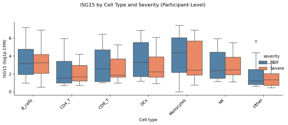
Single-Gene Cross-Sectional Check (Participant-Level)#
Here, we use a focused single-gene comparison to validate cross-sectional differences at the participant level. This avoids pseudoreplication and provides an interpretable effect for one gene in a specific lineage.
[20]:
print("\n=== Single-Gene Cross-Sectional Check (Participant-Level) ===")
gene = "ISG15"
celltypes = sorted(adata.obs["lineage"].dropna().unique())
# Compute participant-level means per celltype and group
gene_name = st.resolve_feature(adata, gene)
# Use log1p-CPM (library-size normalized) to avoid confounding by sequencing depth
expr = st.extract_gene_vector(adata, gene_name, layer="log1p_cpm")
df_expr = adata.obs[["participant_id", "severity", "lineage"]].copy()
df_expr["expr"] = expr
df_part = (
df_expr.groupby(["participant_id", "severity", "lineage"], observed=True)["expr"]
.mean()
.reset_index()
)
# Run per-celltype tests
rows = []
for ct in celltypes:
result, _ = st.compare_gene_in_celltype(
adata,
gene=gene,
celltypes=ct,
group_col="severity",
group1="Severe",
group2="Mild",
participant_col="participant_id",
celltype_col="lineage",
min_cells_per_patient=10,
min_patients_per_group=3,
)
rows.append(result)
df_res = pd.DataFrame(rows)
df_res["celltype"] = df_res["celltypes"].apply(lambda x: x[0] if isinstance(x, list) and len(x) == 1 else str(x))
display(df_res)
# Plot participant-level distributions by celltype
g = sns.catplot(
data=df_part,
x="lineage",
y="expr",
hue="severity",
kind="box",
height=4,
aspect=2.2,
palette={"Mild": "steelblue", "Severe": "coral"},
)
g.set_xticklabels(rotation=45, ha="right")
g.set_axis_labels("Cell type", f"{gene} (log1p CPM)")
g.fig.suptitle(f"{gene} by Cell Type and Severity (Participant-Level)", y=1.05)
plt.tight_layout()
plt.show()
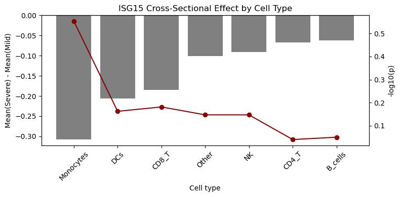
# Barplot of effect sizes with -log10(p) overlay
df_plot = df_res.dropna(subset=["p_value"]).copy()
if not df_plot.empty:
df_plot["neglog10p"] = -np.log10(df_plot["p_value"].clip(lower=1e-12))
df_plot = df_plot.sort_values("delta")
fig, ax1 = plt.subplots(figsize=(8, 4))
ax1.bar(df_plot["celltype"], df_plot["delta"], color="gray")
ax1.axhline(0, color="black", linewidth=0.8)
ax1.set_ylabel("Mean(Severe) - Mean(Mild)")
ax1.set_xlabel("Cell type")
ax1.set_title(f"{gene} Cross-Sectional Effect by Cell Type")
ax1.tick_params(axis="x", rotation=45)
ax2 = ax1.twinx()
ax2.plot(df_plot["celltype"], df_plot["neglog10p"], color="darkred", marker="o")
ax2.set_ylabel("-log10(p)")
plt.tight_layout()
plt.show()
else:
print("No valid p-values available for plotting.")
=== Single-Gene Cross-Sectional Check (Participant-Level) ===
| gene | celltypes | group1 | group2 | n_group1 | n_group2 | mean_group1 | mean_group2 | delta | p_value | celltype | |
|---|---|---|---|---|---|---|---|---|---|---|---|
| 0 | ISG15 | [B_cells] | Severe | Mild | 10 | 23 | 1.055019 | 1.117754 | -0.062736 | 0.890947 | B_cells |
| 1 | ISG15 | [CD4_T] | Severe | Mild | 11 | 23 | 0.349447 | 0.416083 | -0.066635 | 0.912062 | CD4_T |
| 2 | ISG15 | [CD8_T] | Severe | Mild | 11 | 23 | 0.474734 | 0.659512 | -0.184778 | 0.658669 | CD8_T |
| 3 | ISG15 | [DCs] | Severe | Mild | 10 | 21 | 0.699574 | 0.906295 | -0.206721 | 0.688090 | DCs |
| 4 | ISG15 | [Monocytes] | Severe | Mild | 10 | 16 | 0.936911 | 1.244191 | -0.307280 | 0.279944 | Monocytes |
| 5 | ISG15 | [NK] | Severe | Mild | 11 | 23 | 0.480815 | 0.571585 | -0.090770 | 0.712779 | NK |
| 6 | ISG15 | [Other] | Severe | Mild | 11 | 23 | 0.242101 | 0.342777 | -0.100676 | 0.712779 | Other |
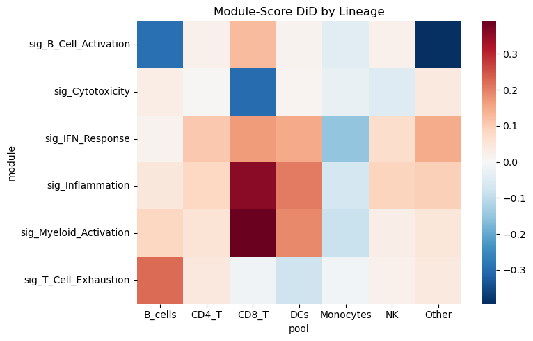
Module-Score Pseudobulk DiD by Lineage#
Here, we collapse each participant×visit×lineage into a pseudobulk mean of module scores, then compute DiD per lineage. This highlights which lineages drive the severity-associated changes.
Note: This dataset has no longitudinally paired participants, so the code falls back to a repeated-cross-sectional (unpaired) OLS DiD. This is a weaker design than a true paired DiD — treat any discoveries as exploratory hypothesis-generating only, not confirmatory.
[21]:
if signature_cols:
    # Choose visit pair with best paired coverage across arms
    visit_levels = sorted(adata.obs["dfo_bin"].dropna().unique())
    best_pair = None
    best_score = -1
    min_per_arm = 2
    for v1, v2 in itertools.combinations(visit_levels, 2):
        wide = (
            adata.obs
            .groupby(["participant_id", "dfo_bin"], observed=True)
            .size()
            .unstack(fill_value=0)
        )
        paired_ids = wide[(wide.get(v1, 0) > 0) & (wide.get(v2, 0) > 0)].index
        if len(paired_ids) == 0:
            continue
        arm_counts = (
            adata.obs[adata.obs["participant_id"].isin(paired_ids)]
            .groupby("severity")["participant_id"]
            .nunique()
        )
        if len(arm_counts) < 2:
            continue
        min_arm = min(arm_counts.get("Severe", 0), arm_counts.get("Mild", 0))
        if min_arm < min_per_arm:
            continue
        if min_arm > best_score:
            best_score = min_arm
            best_pair = (v1, v2)

    allow_unpaired = False
    if best_pair is None:
        print("No visit pair has >=2 paired participants per arm. DiD may be underpowered.")
        visits_pair = tuple(visit_levels[:2])
        allow_unpaired = True
        # Fallback: repeated-cross-sectional OLS DiD (weaker than paired)
    else:
        visits_pair = best_pair
    print("Using visits:", visits_pair)

    # Filter lineages with enough paired participants for the chosen pair
    paired_counts = (
        adata.obs[adata.obs["dfo_bin"].isin(visits_pair)]
        .groupby(["participant_id", "lineage"])["dfo_bin"]
        .nunique()
        .reset_index(name="n_visits")
    )
    paired_lineages = paired_counts[paired_counts["n_visits"] >= 2]["lineage"].value_counts()
    keep_lineages = paired_lineages[paired_lineages >= 2].index.tolist()
    if not keep_lineages:
        keep_lineages = sorted(adata.obs["lineage"].dropna().unique())

    print("Lineages with paired participants:", keep_lineages)

    adata_use = adata[adata.obs["lineage"].isin(keep_lineages)].copy()
    pb_mod = st.module_score_pseudobulk(
        adata_use,
        module_cols=signature_cols,
        design=design,
        visits=visits_pair,
        pool_col="lineage",
        min_cells_per_group=1,
    )
    display(pb_mod.head())

    def _run_mod_did(pb_df, allow_unpaired_flag):
        return st.module_score_did_by_pool(
            pb_df,
            design=design,
            visits=visits_pair,
            min_paired=2,
            n_perm=300,
            seed=SEED,
            fdr_within="module",
            allow_unpaired=allow_unpaired_flag,
        )

    res_mod = _run_mod_did(pb_mod, allow_unpaired)
    if res_mod.empty and not allow_unpaired:
        print("No valid paired lineage-level DiD results. Retrying with unpaired OLS DiD.")
        res_mod = _run_mod_did(pb_mod, True)

    if res_mod.empty:
        print("No valid lineage-level DiD results. Falling back to pooled lineage.")
        pb_all = st.module_score_pseudobulk(
            adata_use,
            module_cols=signature_cols,
            design=design,
            visits=visits_pair,
            pool_map={"All_Lineages": keep_lineages},
            celltype_col="lineage",
            min_cells_per_group=1,
        )
        res_mod = st.module_score_did_by_pool(
            pb_all,
            design=design,
            visits=visits_pair,
            min_paired=2,
            n_perm=300,
            seed=SEED,
            fdr_within=None,
            allow_unpaired=True,
        )

    if not res_mod.empty:
        display(res_mod.sort_values("p_DiD").head(20))
        pivot = res_mod.pivot(index="module", columns="pool", values="beta_DiD")
        plt.figure(figsize=(8, 5))
        sns.heatmap(pivot, cmap="RdBu_r", center=0)
        plt.title("Module-Score DiD by Lineage")
        plt.tight_layout()
        plt.show()
    else:
        print("No valid module-score DiD results after fallback.")
else:
    print("No module scores available for pseudobulk DiD.")
No visit pair has >=2 paired participants per arm. DiD may be underpowered.
Using visits: ('DFO_0-7', 'DFO_15+')
Lineages with paired participants: ['B_cells', 'CD4_T', 'CD8_T', 'DCs', 'Monocytes', 'NK', 'Other']
| participant_id | dfo_bin | severity | pool | module | module_score | n_cells | |
|---|---|---|---|---|---|---|---|
| 0 | AP1 | DFO_15+ | Severe | B_cells | sig_B_Cell_Activation | 0.899969 | 65 |
| 1 | AP1 | DFO_15+ | Severe | B_cells | sig_Cytotoxicity | -0.434286 | 65 |
| 2 | AP1 | DFO_15+ | Severe | B_cells | sig_IFN_Response | -0.220424 | 65 |
| 3 | AP1 | DFO_15+ | Severe | B_cells | sig_Inflammation | -0.356552 | 65 |
| 4 | AP1 | DFO_15+ | Severe | B_cells | sig_Myeloid_Activation | -0.215348 | 65 |
/var/folders/71/dc4p4yz15s74z9c69xy6sk_00000gt/T/ipykernel_52813/2438914800.py:67: UserWarning: FDR correction is applied within each 'module' group (column FDR_DiD). Per-group FDR does not control the overall false discovery rate across all tests. Consult FDR_DiD_global (when fdr_global=True) for a globally corrected q-value.
  return st.module_score_did_by_pool(
| pool | module | mean_delta_treated | mean_delta_control | beta_DiD | p_DiD | p_treated | p_control | n_units | FDR_DiD | FDR_DiD_global | |
|---|---|---|---|---|---|---|---|---|---|---|---|
| 10 | CD4_T | sig_Myeloid_Activation | 0.033539 | -0.022396 | 0.055934 | 0.005882 | 1.448392e-02 | 1.435256e-01 | 18 | 0.041177 | 0.247059 |
| 39 | Other | sig_Inflammation | 0.063717 | -0.031208 | 0.094925 | 0.060188 | 9.327552e-02 | 3.731571e-01 | 18 | 0.421313 | 0.766013 |
| 0 | B_cells | sig_B_Cell_Activation | 0.023480 | 0.316719 | -0.293239 | 0.088852 | 7.913530e-01 | 3.046176e-02 | 18 | 0.287586 | 0.766013 |
| 12 | CD8_T | sig_B_Cell_Activation | 0.084332 | -0.041179 | 0.125511 | 0.090395 | 1.523304e-01 | 3.956929e-01 | 18 | 0.287586 | 0.766013 |
| 36 | Other | sig_B_Cell_Activation | -0.062174 | 0.331806 | -0.393980 | 0.123251 | 7.678999e-01 | 3.764561e-02 | 18 | 0.287586 | 0.766013 |
| 9 | CD4_T | sig_Inflammation | 0.025529 | -0.057104 | 0.082633 | 0.148328 | 5.669148e-01 | 1.350545e-01 | 18 | 0.454691 | 0.766013 |
| 22 | DCs | sig_Myeloid_Activation | 0.342098 | 0.152212 | 0.189887 | 0.163697 | 4.228575e-03 | 4.767019e-02 | 18 | 0.306405 | 0.766013 |
| 40 | Other | sig_Myeloid_Activation | 0.032732 | -0.017220 | 0.049952 | 0.177722 | 2.535658e-01 | 4.907715e-01 | 18 | 0.306405 | 0.766013 |
| 5 | B_cells | sig_T_Cell_Exhaustion | 0.161363 | -0.061513 | 0.222876 | 0.186291 | 2.116081e-01 | 5.922744e-01 | 18 | 0.906840 | 0.766013 |
| 33 | NK | sig_Inflammation | 0.108476 | 0.020518 | 0.087958 | 0.194868 | 2.098862e-02 | 6.833466e-01 | 18 | 0.454691 | 0.766013 |
| 16 | CD8_T | sig_Myeloid_Activation | 0.125039 | -0.265575 | 0.390613 | 0.204761 | 6.135721e-01 | 1.815111e-01 | 18 | 0.306405 | 0.766013 |
| 4 | B_cells | sig_Myeloid_Activation | 0.051348 | -0.035312 | 0.086660 | 0.218861 | 3.390088e-01 | 4.643447e-01 | 18 | 0.306405 | 0.766013 |
| 15 | CD8_T | sig_Inflammation | 0.158589 | -0.197572 | 0.356161 | 0.291135 | 6.090213e-01 | 2.486595e-01 | 18 | 0.509486 | 0.831897 |
| 14 | CD8_T | sig_IFN_Response | -0.576200 | -0.744433 | 0.168233 | 0.304934 | 7.579125e-08 | 3.598030e-09 | 18 | 0.735373 | 0.831897 |
| 38 | Other | sig_IFN_Response | -0.369401 | -0.517339 | 0.147938 | 0.305060 | 4.902311e-09 | 4.886264e-05 | 18 | 0.735373 | 0.831897 |
| 23 | DCs | sig_T_Cell_Exhaustion | 0.103597 | 0.183398 | -0.079801 | 0.316913 | 1.869413e-01 | 7.120731e-09 | 18 | 0.906840 | 0.831897 |
| 3 | B_cells | sig_Inflammation | -0.011181 | -0.056999 | 0.045818 | 0.405382 | 7.451818e-01 | 1.890339e-01 | 18 | 0.567535 | 0.872738 |
| 25 | Monocytes | sig_Cytotoxicity | -0.039196 | -0.010555 | -0.028641 | 0.409974 | 1.599962e-01 | 6.386748e-01 | 18 | 0.967076 | 0.872738 |
| 13 | CD8_T | sig_Cytotoxicity | -0.280668 | 0.020925 | -0.301593 | 0.429210 | 4.224859e-01 | 9.143946e-01 | 18 | 0.967076 | 0.872738 |
| 11 | CD4_T | sig_T_Cell_Exhaustion | 0.049772 | 0.007516 | 0.042256 | 0.439720 | 2.531214e-01 | 8.332307e-01 | 18 | 0.906840 | 0.872738 |
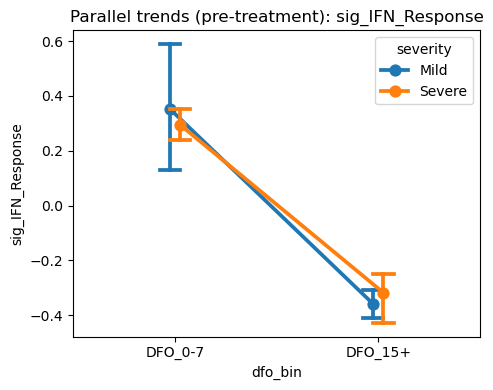
Parallel Trends Visualization (Early Visits)#
Here we visualize pre-treatment trends across early visits to assess whether arms move in parallel before divergence. This is a diagnostic, not a formal test.
[22]:
if signature_cols:
    try:
        st.plot_parallel_trends(
            adata,
            feature=signature_cols[0],
            design=design,
            visits=visits_pair,
        )
        plt.tight_layout()
        plt.show()
    except Exception as e:
        print(f'Parallel trends plot skipped: {e}')